Reference
Accessor Methods
The following methods are available via traja.accessor.TrajaAccessor:
- class traja.accessor.TrajaAccessor(pandas_obj)[source]
Accessor for pandas DataFrame with trajectory-specific numerical and analytical functions.
Access with df.traja.
- property center
Return the center point of this trajectory.
- property bounds
Return limits of x and y dimensions (
(xmin, xmax), (ymin, ymax)).
- _get_time_col()[source]
Returns time column in trajectory.
Args:
- Returns
name of time column, ‘index’ or None
- Return type
time_col (str or None)
- between(begin: str, end: str)[source]
Returns trajectory between begin and end` if time column is datetime64.
- Parameters
- Returns
Dataframe between values.
- Return type
trj (
TrajaDataFrame)
>>> s = pd.to_datetime(pd.Series(['Jun 30 2000 12:00:01', 'Jun 30 2000 12:00:02', 'Jun 30 2000 12:00:03']))
>>> df = traja.TrajaDataFrame({'x':[0,1,2],'y':[1,2,3],'time':s})
>>> df.traja.between('12:00:00','12:00:01')
                 time  x  y
0 2000-06-30 12:00:01  0  1
- resample_time(step_time: float)[source]
Returns trajectory resampled with
step_time.- Parameters
step_time (float) – Step time
- Returns
Dataframe resampled.
- Return type
trj (
TrajaDataFrame)
- rediscretize_points(R, **kwargs)[source]
Rediscretize points
- trip_grid(bins: Union[int, tuple] = 10, log: bool = False, spatial_units=None, normalize: bool = False, hist_only: bool = False, plot: bool = True, **kwargs)[source]
Returns a 2D histogram of trip.
- Parameters
- Returns
2D histogram as array image (
matplotlib.collections.PathCollection: image of histogram- Return type
hist (
numpy.ndarray)
- plot(n_coords: Optional[int] = None, show_time=False, **kwargs)[source]
Plot trajectory over period.
- Parameters
n_coords (int) – Number of coordinates to plot
**kwargs – additional keyword arguments to
matplotlib.axes.Axes.scatter()
- Returns
Axes of plot
- Return type
ax (
Axes)
- plot_3d(**kwargs)[source]
Plot 3D trajectory for single identity over period.
Args: trj (
traja.TrajaDataFrame): trajectory n_coords (int, optional): Number of coordinates to plot **kwargs: additional keyword arguments tomatplotlib.axes.Axes.scatter()- Returns
collection that was plotted
- Return type
collection (
PathCollection)
Note
Takes a while to plot large trajectories. Consider using first:
rt = trj.traja.rediscretize(R=1.) # Replace R with appropriate step length
rt.traja.plot_3d()
- plot_flow(kind='quiver', **kwargs)[source]
Plot grid cell flow.
- Parameters
kind (str) – Kind of plot (eg, ‘quiver’,’surface’,’contour’,’contourf’,’stream’)
**kwargs – additional keyword arguments to
matplotlib.axes.Axes.scatter()
- Returns
Axes of plot
- Return type
ax (
Axes)
- plot_collection(colors=None, **kwargs)[source]
- apply_all(method, id_col=None, **kwargs)[source]
Applies method to all trajectories and returns grouped dataframes or series
- property xy
Returns a
numpy.ndarrayof x,y coordinates.- Parameters
split (bool) – Split into seaprate x and y
numpy.ndarrays- Returns
xy (
numpy.ndarray) – x,y coordinates (separate if split is True)
>>> df = traja.TrajaDataFrame({'x':[0,1,2],'y':[1,2,3]})
>>> df.traja.xy
array([[0, 1],
       [1, 2],
       [2, 3]])
- _check_has_time()[source]
Check for presence of displacement time column.
- __getattr__(name)[source]
Catch all method calls which are not defined and forward to modules.
- transitions(*args, **kwargs)[source]
Calculate transition matrix
- calc_derivatives(assign: bool = False)[source]
Returns derivatives displacement and displacement_time.
- Parameters
assign (bool) – Assign output to
TrajaDataFrame(Default value = False)- Returns
Derivatives.
- Return type
derivs (
OrderedDict)
>>> df = traja.TrajaDataFrame({'x':[0,1,2],'y':[1,2,3],'time':[0., 0.2, 0.4]})
>>> df.traja.calc_derivatives()
   displacement  displacement_time
0           NaN                0.0
1      1.414214                0.2
2      1.414214                0.4
- speed_intervals(faster_than: Optional[Union[float, int]] = None, slower_than: Optional[Union[float, int]] = None)[source]
Returns
TrajaDataFramewith speed time intervals.Returns a dataframe of time intervals where speed is slower and/or faster than specified values.
- Parameters
- Returns
result (
DataFrame) – time intervals as dataframe
Note
Implementation ported to Python, heavily inspired by Jim McLean’s trajr package.
- to_shapely()[source]
Returns shapely object for area, bounds, etc. functions.
Args:
- Returns
Shapely shape.
- Return type
shape (shapely.geometry.linestring.LineString)
>>> df = traja.TrajaDataFrame({'x':[0,1,2],'y':[1,2,3]})
>>> shape = df.traja.to_shapely()
>>> shape.is_closed
False
- calc_displacement(assign: bool = True) Series[source]
Returns
Seriesof float with displacement between consecutive indices.- Parameters
assign (bool, optional) – Assign displacement to TrajaAccessor (Default value = True)
- Returns
Displacement series.
- Return type
displacement (
pandas.Series)
>>> df = traja.TrajaDataFrame({'x':[0,1,2],'y':[1,2,3]})
>>> df.traja.calc_displacement()
0         NaN
1    1.414214
2    1.414214
Name: displacement, dtype: float64
- calc_angle(assign: bool = True) Series[source]
Returns
Serieswith angle between steps as a function of displacement with regard to x axis.- Parameters
assign (bool, optional) – Assign turn angle to TrajaAccessor (Default value = True)
- Returns
Angle series.
- Return type
angle (
pandas.Series)
>>> df = traja.TrajaDataFrame({'x':[0,1,2],'y':[1,2,3]})
>>> df.traja.calc_angle()
0     NaN
1    45.0
2    45.0
dtype: float64
- scale(scale: float, spatial_units: str = 'm')[source]
Scale trajectory when converting, eg, from pixels to meters.
- Parameters
scale (float) – Scale to convert coordinates
spatial_units (str., optional) – Spatial units (eg, ‘m’) (Default value = “m”)
>>> df = traja.TrajaDataFrame({'x':[0,1,2],'y':[1,2,3]})
>>> df.traja.scale(0.1)
>>> df
     x    y
0  0.0  0.1
1  0.1  0.2
2  0.2  0.3
- rediscretize(R: float)[source]
Resample a trajectory to a constant step length. R is rediscretized step length.
- Parameters
R (float) – Rediscretized step length (eg, 0.02)
- Returns
rediscretized trajectory
- Return type
rt (
traja.TrajaDataFrame)
Note
Based on the appendix in Bovet and Benhamou, (1988) and Jim McLean’s trajr implementation.
>>> df = traja.TrajaDataFrame({'x':[0,1,2],'y':[1,2,3]})
>>> df.traja.rediscretize(1.)
          x         y
0  0.000000  1.000000
1  0.707107  1.707107
2  1.414214  2.414214
- grid_coordinates(**kwargs)[source]
- calc_heading(assign: bool = True)[source]
Calculate trajectory heading.
- Parameters
assign (bool) – (Default value = True)
- Returns
heading as a
Series- Return type
heading (
pandas.Series)
..doctest:
>>> df = traja.TrajaDataFrame({'x':[0,1,2],'y':[1,2,3]})
>>> df.traja.calc_heading()
0     NaN
1    45.0
2    45.0
Name: heading, dtype: float64
- calc_turn_angle(assign: bool = True)[source]
Calculate turn angle.
- Parameters
assign (bool) – (Default value = True)
- Returns
Turn angle
- Return type
turn_angle (
Series)
>>> df = traja.TrajaDataFrame({'x':[0,1,2],'y':[1,2,3]})
>>> df.traja.calc_turn_angle()
0    NaN
1    NaN
2    0.0
Name: turn_angle, dtype: float64
Plotting functions
The following methods are available via traja.plotting:
- plotting.animate(polar: bool = True, save: bool = False)
Animate trajectory.
- Parameters
- Returns
animation
- Return type
- plotting.bar_plot(bins: Optional[Union[int, tuple]] = None, **kwargs) Axes
Plot trajectory for single animal over period.
- Parameters
- Returns
Axes of plot
- Return type
ax (
PathCollection)
- plotting.color_dark(ax: Optional[Axes] = None, start: int = 19, end: int = 7)
Color dark phase in plot. :param series: :type series: pd.Series :param ax (: class: ~matplotlib.axes.Axes): axis to plot on (eg, plt.gca()) :param start: start of dark period/night :type start: int :param end: end of dark period/day :type end: hour
- Returns
Axes of plot
- Return type
ax (
AxesSubplot)
- plotting.fill_ci(window: Union[int, str]) Figure
Fill confidence interval defined by SEM over mean of window. Window can be interval or offset, eg, ’30s’.
- plotting.find_runs() -> (<class 'numpy.ndarray'>, <class 'numpy.ndarray'>, <class 'numpy.ndarray'>)
Find runs of consecutive items in an array. From https://gist.github.com/alimanfoo/c5977e87111abe8127453b21204c1065.
- plotting.plot(n_coords: Optional[int] = None, show_time: bool = False, accessor: Optional[TrajaAccessor] = None, ax=None, **kwargs) PathCollection
Plot trajectory for single animal over period.
- Parameters
trj (
traja.TrajaDataFrame) – trajectoryn_coords (int, optional) – Number of coordinates to plot
show_time (bool) – Show colormap as time
accessor (
TrajaAccessor, optional) – TrajaAccessor instanceax (
Axes) – axes for plottinginteractive (bool) – show plot immediately
**kwargs – additional keyword arguments to
matplotlib.axes.Axes.scatter()
- Returns
collection that was plotted
- Return type
collection (
PathCollection)
- plotting.plot_3d(**kwargs) PathCollection
Plot 3D trajectory for single identity over period.
- Parameters
trj (
traja.TrajaDataFrame) – trajectoryn_coords (int, optional) – Number of coordinates to plot
**kwargs – additional keyword arguments to
matplotlib.axes.Axes.scatter()
- Returns
Axes of plot
- Return type
ax (
PathCollection)
Note
Takes a while to plot large trajectories. Consider using first:
rt = trj.traja.rediscretize(R=1.) # Replace R with appropriate step length
rt.traja.plot_3d()
- plotting.plot_actogram(dark=(19, 7), ax: Optional[Axes] = None, **kwargs)
Plot activity or displacement as an actogram.
Note
For published example see Eckel-Mahan K, Sassone-Corsi P. Phenotyping Circadian Rhythms in Mice. Curr Protoc Mouse Biol. 2015;5(3):271-281. Published 2015 Sep 1. doi:10.1002/9780470942390.mo140229
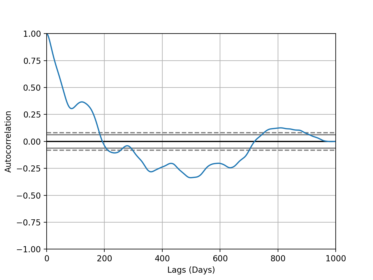
- plotting.plot_autocorrelation(coord: str = 'y', unit: str = 'Days', xmax: int = 1000, interactive: bool = True)
Plot autocorrelation of given coordinate.
- Parameters
Trajectory (trj -) –
'y' (coord - 'x' or) –
string (unit -) –
eg –
'Days' –
value (xmax - max xaxis) –
immediately (interactive - Plot) –
- Returns
Matplotlib Figure
(Source code, png, hires.png, pdf)
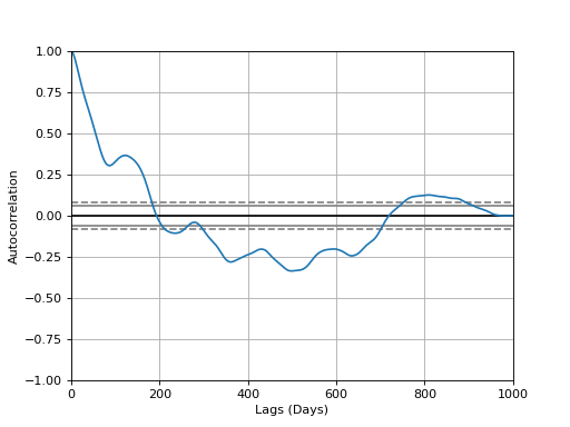
Note
Convenience wrapper for pandas
autocorrelation_plot().
- plotting.plot_contour(bins: Optional[Union[int, tuple]] = None, filled: bool = True, quiver: bool = True, contourplot_kws: dict = {}, contourfplot_kws: dict = {}, quiverplot_kws: dict = {}, ax: Optional[Axes] = None, **kwargs) Axes
Plot average flow from each grid cell to neighbor.
- Parameters
trj – Traja DataFrame
bins (int or tuple) – Tuple of x,y bin counts; if bins is int, bin count of x, with y inferred from aspect ratio
filled (bool) – Contours filled
quiver (bool) – Quiver plot
contourplot_kws – Additional keyword arguments for
contour()contourfplot_kws – Additional keyword arguments for
contourf()quiverplot_kws – Additional keyword arguments for
quiver()ax (optional) – Matplotlib Axes
- Returns
Axes of quiver plot
- Return type
ax (
Axes)
- plotting.plot_clustermap(rule: Optional[str] = None, nr_steps=None, colors: Optional[List[Union[int, str]]] = None, **kwargs)
Plot cluster map / dendrogram of trajectories with DatetimeIndex.
- Parameters
displacements – list of pd.Series, outputs of
traja.calc_displacement()rule – how to resample series, eg ’30s’ for 30-seconds
nr_steps – select first N samples for clustering
colors – list of colors (eg, ‘b’,’r’) to map to each trajectory
kwargs – keyword arguments for
seaborn.clustermap()
- Returns
a
seaborn.matrix.ClusterGrid()instance- Return type
cg
Note
Requires seaborn to be installed. Install it with ‘pip install seaborn’.
- plotting.plot_flow(kind: str = 'quiver', *args, contourplot_kws: dict = {}, contourfplot_kws: dict = {}, streamplot_kws: dict = {}, quiverplot_kws: dict = {}, surfaceplot_kws: dict = {}, **kwargs) Figure
Plot average flow from each grid cell to neighbor.
- Parameters
bins (int or tuple) – Tuple of x,y bin counts; if bins is int, bin count of x, with y inferred from aspect ratio
kind (str) – Choice of ‘quiver’,’contourf’,’stream’,’surface’. Default is ‘quiver’.
contourplot_kws – Additional keyword arguments for
contour()contourfplot_kws – Additional keyword arguments for
contourf()streamplot_kws – Additional keyword arguments for
streamplot()quiverplot_kws – Additional keyword arguments for
quiver()surfaceplot_kws – Additional keyword arguments for
plot_surface()
- Returns
Axes of plot
- Return type
ax (
Axes)
- plotting.plot_quiver(bins: Optional[Union[int, tuple]] = None, quiverplot_kws: dict = {}, **kwargs) Axes
Plot average flow from each grid cell to neighbor.
- plotting.plot_stream(bins: Optional[Union[int, tuple]] = None, cmap: str = 'viridis', contourfplot_kws: dict = {}, contourplot_kws: dict = {}, streamplot_kws: dict = {}, **kwargs) Figure
Plot average flow from each grid cell to neighbor.
- Parameters
bins (int or tuple) – Tuple of x,y bin counts; if bins is int, bin count of x, with y inferred from aspect ratio
contourplot_kws – Additional keyword arguments for
contour()contourfplot_kws – Additional keyword arguments for
contourf()streamplot_kws – Additional keyword arguments for
streamplot()
- Returns
Axes of stream plot
- Return type
ax (
Axes)
- plotting.plot_surface(bins: Optional[Union[int, tuple]] = None, cmap: str = 'viridis', **surfaceplot_kws: dict) Figure
Plot surface of flow from each grid cell to neighbor in 3D.
- plotting.plot_transition_matrix(interactive=True, **kwargs) AxesImage
Plot transition matrix.
- Parameters
data (trajectory or square transition matrix) –
interactive (bool) – show plot
kwargs – kwargs to
traja.grid_coordinates()
- Returns
axesimage (matplotlib.image.AxesImage)
- plotting.plot_xy(*args: Optional, **kwargs: Optional)
Plot trajectory from xy values.
- Parameters
xy (np.ndarray) – xy values of dimensions N x 2
*args – Plot args
**kwargs – Plot kwargs
- plotting.polar_bar(feature: str = 'turn_angle', bin_size: int = 2, threshold: float = 0.001, overlap: bool = True, ax: Optional[Axes] = None, **plot_kws: str) Axes
Plot polar bar chart.
- Parameters
- Returns
Axes of plot
- Return type
ax (
PathCollection)
- plotting.plot_prediction(dataloader, index, scaler=None)
- plotting.sans_serif()
Convenience function for changing plot text to serif font.
- plotting.stylize_axes()
Add top and right border to plot, set ticks.
- plotting.trip_grid(bins: Union[tuple, int] = 10, log: bool = False, spatial_units: Optional[str] = None, normalize: bool = False, hist_only: bool = False, **kwargs) Tuple[ndarray, PathCollection]
Generate a heatmap of time spent by point-to-cell gridding.
- Parameters
- Returns
2D histogram as array image (
matplotlib.collections.PathCollection: image of histogram- Return type
hist (
numpy.ndarray)
Analysis
The following methods are available via traja.trajectory:
- trajectory.calc_angle(unit: str = 'degrees', lag: int = 1)
Returns a
Serieswith angle between steps as a function of displacement with regard to x axis.- Parameters
- Returns
Angle series.
- Return type
angle (
pandas.Series)
- trajectory.calc_convex_hull() array
Identify containing polygonal convex hull for full Trajectory Interior points filtered with
traja.trajectory.inside()method, takes quadrilateral using extrema points (minx, maxx, miny, maxy) - convex hull points MUST all be outside such a polygon. Returns an array with all points in the convex hull.Implementation of Graham Scan technique <https://en.wikipedia.org/wiki/Graham_scan>_.
- Returns
n x 2 (x,y) array
- Return type
point_arr (
ndarray)
>> #Quick visualizaation
>> import matplotlib.pyplot as plt
>> df = traja.generate(n=10000, convex_hull=True)
>> xs, ys = [*zip(*df.convex_hull)]
>> _ = plt.plot(df.x.values, df.y.values, 'o', 'blue')
>> _ = plt.plot(xs, ys, '-o', color='red')
>> _ = plt.show()
Note
Incorporates Akl-Toussaint method for filtering interior points.
Note
Performative loss beyond ~100,000-200,000 points, algorithm has O(nlogn) complexity.
- trajectory.calc_derivatives()
Returns derivatives
displacementanddisplacement_timeas DataFrame.- Parameters
trj (
TrajaDataFrame) – Trajectory- Returns
Derivatives.
- Return type
derivs (
DataFrame)
>>> df = traja.TrajaDataFrame({'x':[0,1,2],'y':[1,2,3],'time':[0., 0.2, 0.4]})
>>> traja.calc_derivatives(df)
   displacement  displacement_time
0           NaN                0.0
1      1.414214                0.2
2      1.414214                0.4
- trajectory.calc_displacement(lag=1)
Returns a
Seriesoffloatdisplacement between consecutive indices.- Parameters
trj (
TrajaDataFrame) – Trajectorylag (int) – time steps between displacement calculation
- Returns
Displacement series.
- Return type
displacement (
pandas.Series)
>>> df = traja.TrajaDataFrame({'x':[0,1,2],'y':[1,2,3]})
>>> traja.calc_displacement(df)
0         NaN
1    1.414214
2    1.414214
Name: displacement, dtype: float64
- trajectory.calc_heading()
Calculate trajectory heading.
- Parameters
trj (
TrajaDataFrame) – Trajectory- Returns
heading as a
Series- Return type
heading (
pandas.Series)
..doctest:
>>> df = traja.TrajaDataFrame({'x':[0,1,2],'y':[1,2,3]})
>>> traja.calc_heading(df)
0     NaN
1    45.0
2    45.0
Name: heading, dtype: float64
- trajectory.calc_turn_angle()
Return a
Seriesof floats with turn angles.- Parameters
trj (
traja.frame.TrajaDataFrame) – Trajectory- Returns
Turn angle
- Return type
turn_angle (
Series)
>>> df = traja.TrajaDataFrame({'x':[0,1,2],'y':[1,2,3]})
>>> traja.calc_turn_angle(df)
0    NaN
1    NaN
2    0.0
Name: turn_angle, dtype: float64
- trajectory.calc_flow_angles()
Calculate average flow between grid indices.
- trajectory.cartesian_to_polar() -> (<class 'float'>, <class 'float'>)
Convert
numpy.ndarrayxyto polar coordinatesrandtheta.- Parameters
xy (
numpy.ndarray) – x,y coordinates- Returns
step-length and angle
- Return type
- trajectory.coords_to_flow(bins: Optional[Union[int, tuple]] = None)
Calculate grid cell flow from trajectory.
- trajectory.determine_colinearity(p1: ndarray, p2: ndarray)
Determine whether trio of points constitute a right turn, or whether they are left turns (or colinear/straight line).
- trajectory.distance_between(B: TrajaDataFrame, method='dtw')
Returns distance between two trajectories.
- trajectory.distance() float
Calculates the distance from start to end of trajectory, also called net distance, displacement, or bee-line from start to finish.
- Parameters
trj (
TrajaDataFrame) – Trajectory- Returns
distance (float)
>> df = traja.generate()
>> traja.distance(df)
117.01507823153617
- trajectory.euclidean(v, w=None)
Computes the Euclidean distance between two 1-D arrays.
The Euclidean distance between 1-D arrays u and v, is defined as
\[ \begin{align}\begin{aligned}{||u-v||}_2\\\left(\sum{(w_i |(u_i - v_i)|^2)}\right)^{1/2}\end{aligned}\end{align} \]- Parameters
u ((N,) array_like) – Input array.
v ((N,) array_like) – Input array.
w ((N,) array_like, optional) – The weights for each value in u and v. Default is None, which gives each value a weight of 1.0
- Returns
euclidean – The Euclidean distance between vectors u and v.
- Return type
double
Examples
>>> from scipy.spatial import distance
>>> distance.euclidean([1, 0, 0], [0, 1, 0])
1.4142135623730951
>>> distance.euclidean([1, 1, 0], [0, 1, 0])
1.0
- trajectory.expected_sq_displacement(n: int = 0, eqn1: bool = True) float
Expected displacement.
Note
This method is experimental and needs testing.
- trajectory.fill_in_traj()
- trajectory.from_xy()
Convenience function for initializing
TrajaDataFramewith x,y coordinates.- Parameters
xy (
numpy.ndarray) – x,y coordinates- Returns
Trajectory as dataframe
- Return type
traj_df (
TrajaDataFrame)
>>> import numpy as np
>>> xy = np.array([[0,1],[1,2],[2,3]])
>>> traja.from_xy(xy)
   x  y
0  0  1
1  1  2
2  2  3
- trajectory.generate(random: bool = True, step_length: int = 2, angular_error_sd: float = 0.5, angular_error_dist: Optional[Callable] = None, linear_error_sd: float = 0.2, linear_error_dist: Optional[Callable] = None, fps: float = 50, spatial_units: str = 'm', seed: Optional[int] = None, convex_hull: bool = False, **kwargs)
Generates a trajectory.
If
randomisTrue, the trajectory will be a correlated random walk/idiothetic directed walk (Kareiva & Shigesada, 1983), corresponding to an animal navigating without a compass (Cheung, Zhang, Stricker, & Srinivasan, 2008). IfrandomisFalse, it will be(np.ndarray) a directed walk/allothetic directed walk/oriented path, corresponding to an animal navigating with a compass (Cheung, Zhang, Stricker, & Srinivasan, 2007, 2008).By default, for both random and directed walks, errors are normally distributed, unbiased, and independent of each other, so are simple directed walks in the terminology of Cheung, Zhang, Stricker, & Srinivasan, (2008). This behaviour may be modified by specifying alternative values for the
angular_error_distand/orlinear_error_distparameters.The initial angle (for a random walk) or the intended direction (for a directed walk) is
0radians. The starting position is(0, 0).- Parameters
n (int) – (Default value = 1000)
random (bool) – (Default value = True)
step_length – (Default value = 2)
angular_error_sd (float) – (Default value = 0.5)
angular_error_dist (Callable) – (Default value = None)
linear_error_sd (float) – (Default value = 0.2)
linear_error_dist (Callable) – (Default value = None)
fps (float) – (Default value = 50)
convex_hull (bool) – (Default value = False)
spatial_units – (Default value = ‘m’)
**kwargs – Additional arguments
- Returns
Trajectory
- Return type
trj (
traja.frame.TrajaDataFrame)
Note
Based on Jim McLean’s trajr, ported to Python.
Reference: McLean, D. J., & Skowron Volponi, M. A. (2018). trajr: An R package for characterisation of animal trajectories. Ethology, 124(6), 440-448. https://doi.org/10.1111/eth.12739.
- trajectory.get_derivatives()
Returns derivatives
displacement,displacement_time,speed,speed_times,acceleration,acceleration_timesas dictionary.- Parameters
trj (
TrajaDataFrame) – Trajectory- Returns
Derivatives
- Return type
derivs (
DataFrame)
>> df = traja.TrajaDataFrame({'x':[0,1,2],'y':[1,2,3],'time':[0.,0.2,0.4]})
>> df.traja.get_derivatives()
   displacement  displacement_time     speed  speed_times  acceleration  acceleration_times
0           NaN                0.0       NaN          NaN           NaN                 NaN
1      1.414214                0.2  7.071068          0.2           NaN                 NaN
2      1.414214                0.4  7.071068          0.4           0.0                 0.4
- trajectory.grid_coordinates(bins: Optional[Union[int, tuple]] = None, xlim: Optional[tuple] = None, ylim: Optional[tuple] = None, assign: bool = False)
Returns
DataFrameof trajectory discretized into 2D lattice grid coordinates. :param trj: Trajectory :type trj: ~`traja.frame.TrajaDataFrame` :param bins: :type bins: tuple or int :param xlim: :type xlim: tuple :param ylim: :type ylim: tuple :param assign: Return updated original dataframe :type assign: bool- Returns
Trajectory is assign=True otherwise pd.DataFrame
- Return type
trj (TrajaDataFrame`)
- trajectory.inside(bounds_xs: list, bounds_ys: list, minx: float, maxx: float, miny: float, maxy: float)
Determine whether point lies inside or outside of polygon formed by “extrema” points - minx, maxx, miny, maxy. Optimized to be run as broadcast function in numpy along axis.
- Parameters
pt (
ndarray) – Point to test whether inside or outside polygonbounds_xs (list or tuple) – x-coordinates of polygon vertices, in sequence
bounds_ys (list or tuple) – y-coordinates of polygon vertices, same sequence
minx (float) – minimum x coordinate value
maxx (float) – maximum x coordinate value
miny (float) – minimum y coordinate value
maxy (float) – maximum y coordinate value
- Returns
(bool)
Note
Ported to Python from C implementation by W. Randolph Franklin (WRF): <https://wrf.ecse.rpi.edu/Research/Short_Notes/pnpoly.html>
Boolean return “True” for OUTSIDE polygon, meaning it is within subset of possible convex hull coordinates.
- trajectory.length() float
Calculates the cumulative length of a trajectory.
- Parameters
trj (
TrajaDataFrame) – Trajectory- Returns
length (float)
>> df = traja.generate()
>> traja.length(df)
2001.142339606066
- trajectory.polar_to_z(theta: float) complex
Converts polar coordinates
randthetato complex numberz.
- trajectory.rediscretize_points(R: Union[float, int], time_out=False)
Returns a
TrajaDataFramerediscretized to a constant step length R.- Parameters
- Returns
rediscretized trajectory
- Return type
rt (
numpy.ndarray)
- trajectory.resample_time(step_time: str, new_fps: Optional[bool] = None)
Returns a
TrajaDataFrameresampled to consistent step_time intervals.step_timeshould be expressed as a number-time unit combination, eg “2S” for 2 seconds and “2100L” for 2100 milliseconds.- Parameters
- Results:
trj (
TrajaDataFrame): Trajectory
>>> from traja import generate, resample_time
>>> df = generate()
>>> resampled = resample_time(df, '50L') # 50 milliseconds
>>> resampled.head()
                                 x         y
time
1970-01-01 00:00:00.000   0.000000  0.000000
1970-01-01 00:00:00.050   0.919113  4.022971
1970-01-01 00:00:00.100  -1.298510  5.423373
1970-01-01 00:00:00.150  -6.057524  4.708803
1970-01-01 00:00:00.200 -10.347759  2.108385
- trajectory.return_angle_to_point(p0: ndarray)
Calculate angle of points as coordinates in relation to each other. Designed to be broadcast across all trajectory points for a single origin point p0.
- Parameters
p1 (np.ndarray) – Test point [x,y]
p0 (np.ndarray) – Origin/source point [x,y]
- Returns
r (float)
- trajectory.rotate(angle: Union[float, int] = 0, origin: Optional[tuple] = None)
Returns a
TrajaDataFrameRotate a trajectory angle in radians.- Parameters
trj (
traja.frame.TrajaDataFrame) – Trajectoryangle (float) – angle in radians
origin (tuple. optional) – rotate around point (x,y)
- Returns
Trajectory
- Return type
trj (
traja.frame.TrajaDataFrame)
Note
Based on Lyle Scott’s implementation.
- trajectory.smooth_sg(w: Optional[int] = None, p: int = 3)
Returns
DataFrameof trajectory after Savitzky-Golay filtering.- Parameters
- Returns
Trajectory
- Return type
trj (
TrajaDataFrame)
>> df = traja.generate()
>> traja.smooth_sg(df, w=101).head()
           x          y  time
0 -11.194803  12.312742  0.00
1 -10.236337  10.613720  0.02
2  -9.309282   8.954952  0.04
3  -8.412910   7.335925  0.06
4  -7.546492   5.756128  0.08
- trajectory.speed_intervals(faster_than: Optional[float] = None, slower_than: Optional[float] = None) DataFrame
Calculate speed time intervals.
Returns a dictionary of time intervals where speed is slower and/or faster than specified values.
- Parameters
- Returns
result (
DataFrame) – time intervals as dataframe
Note
Implementation ported to Python, heavily inspired by Jim McLean’s trajr package.
>> df = traja.generate()
>> intervals = traja.speed_intervals(df, faster_than=100)
>> intervals.head()
   start_frame  start_time  stop_frame  stop_time  duration
0            1        0.02           3       0.06      0.04
1            4        0.08           8       0.16      0.08
2           10        0.20          11       0.22      0.02
3           12        0.24          15       0.30      0.06
4           17        0.34          18       0.36      0.02
- trajectory.step_lengths()
Length of the steps of
trj.- Parameters
trj (
TrajaDataFrame) – Trajectory
- trajectory.to_shapely()
Returns shapely object for area, bounds, etc. functions.
- Parameters
trj (
TrajaDataFrame) – Trajectory- Returns
shapely.geometry.linestring.LineString – Shapely shape.
>>> df = traja.TrajaDataFrame({'x':[0,1,2],'y':[1,2,3]})
>>> shape = traja.to_shapely(df)
>>> shape.is_closed
False
- trajectory.traj_from_coords(x_col=1, y_col=2, time_col: Optional[str] = None, fps: Union[float, int] = 4, spatial_units: str = 'm', time_units: str = 's') TrajaDataFrame
Create TrajaDataFrame from coordinates.
- Parameters
track – N x 2 numpy array or pandas DataFrame with x and y columns
x_col – column index or x column name
y_col – column index or y column name
time_col – name of time column
fps – Frames per seconds
spatial_units – default m, optional
time_units – default s, optional
- Returns
TrajaDataFrame
- Return type
trj
>> xy = np.random.random((1000, 2))
>> trj = traja.traj_from_coord(xy)
>> assert trj.shape == (1000,4) # columns x, y, time, dt
- trajectory.transition_matrix()
Returns
np.ndarrayof Markov transition probability matrix for grid cell transitions.- Parameters
grid_indices1D (
np.ndarray) –- Returns
M (
numpy.ndarray)
- trajectory.transitions(**kwargs)
Get first-order Markov model for transitions between grid cells.
- Parameters
trj (trajectory) –
kwargs – kwargs to
traja.grid_coordinates()
io functions
The following methods are available via traja.parsers:
- parsers.read_file(id: Optional[str] = None, xcol: Optional[str] = None, ycol: Optional[str] = None, parse_dates: Union[str, bool] = False, xlim: Optional[tuple] = None, ylim: Optional[tuple] = None, spatial_units: str = 'm', fps: Optional[float] = None, **kwargs)
Convenience method wrapping pandas read_csv and initializing metadata.
- Parameters
filepath (str) – path to csv file with x, y and time (optional) columns
id (str) – id for trajectory
xcol (str) – name of column containing x coordinates
ycol (str) – name of column containing y coordinates
parse_dates (Union[list,bool]) – The behavior is as follows: - boolean. if True -> try parsing the index. - list of int or names. e.g. If [1, 2, 3] -> try parsing columns 1, 2, 3 each as a separate date column.
xlim (tuple) – x limits (min,max) for plotting
ylim (tuple) – y limits (min,max) for plotting
spatial_units (str) – for plotting (eg, ‘cm’)
fps (float) – for time calculations
**kwargs – Additional arguments for
pandas.read_csv().
- Returns
Trajectory
- Return type
traj_df (
TrajaDataFrame)
- parsers.from_df(xcol=None, ycol=None, time_col=None, **kwargs)
Returns a
traja.frame.TrajaDataFramefrom apandas DataFrame.- Parameters
df (
pandas.DataFrame) – Trajectory as pandasDataFramexcol (str) –
ycol (str) –
timecol (str) –
- Returns
Trajectory
- Return type
traj_df (
TrajaDataFrame)
>>> df = pd.DataFrame({'x':[0,1,2],'y':[1,2,3]})
>>> traja.from_df(df)
   x  y
0  0  1
1  1  2
2  2  3
TrajaDataFrame
A TrajaDataFrame is a tabular data structure that contains x, y, and time columns.
All pandas DataFrame methods are also available, although they may
not operate in a meaningful way on the x, y, and time columns.
Inheritance diagram:

TrajaCollection
A TrajaCollection holds multiple trajectories for analyzing and comparing trajectories.
It has limited accessibility to lower-level methods.
- class traja.frame.TrajaCollection(trjs: Union[TrajaDataFrame, DataFrame, dict], id_col: Optional[str] = None, **kwargs)[source]
Collection of trajectories.
API Pages
|
A TrajaDataFrame object is a subclass of pandas |
|
Collection of trajectories. |
|
Convenience method wrapping pandas read_csv and initializing metadata. |