Predicting Trajectories
Predicting trajectories with traja can be done with a recurrent neural network (RNN). Traja includes the Long Short Term Memory (LSTM), LSTM Autoencoder (LSTM AE) and LSTM Variational Autoencoder (LSTM VAE) RNNs. Traja also supports custom RNNs.
To model a trajectory using RNNs, one needs to fit the network to the model. Traja includes the MultiTaskRNNTrainer that can solve a prediction, classification and regression problem with traja DataFrames.
Traja also includes a DataLoader that handles traja dataframes.
Below is an example with a prediction LSTM via traja.models.predictive_models.lstm.LSTM.
import traja

df = traja.dataset.example.jaguar()
Note
LSTMs work better with data between -1 and 1. Therefore the data loader scales the data.
batch_size = 10 # How many sequences to train every step. Constrained by GPU memory.
num_past = 10 # How many time steps from which to learn the time series
num_future = 10 # How many time steps to predict
split_by_id = False # Whether to split data into training, test and validation sets based on
                    # the animal's ID or not. If True, an animal's entire trajectory will only
                    # be used for training, or only for testing and so on.
                    # If your animals are territorial (like Jaguars) and you want to forecast
                    # their trajectories, you want this to be false. If, however, you want to
                    # classify the group membership of an animal, you want this to be true,
                    # so that you can verify that previously unseen animals get assigned to
                    # the correct class.
- class traja.models.predictive_models.lstm.LSTM(input_size: int, hidden_size: int, output_size: int, num_future: int = 8, batch_size: int = 8, num_layers: int = 1, reset_state: bool = True, bidirectional: bool = False, dropout: float = 0, batch_first: bool = True)[source]
Deep LSTM network. This implementation returns output_size outputs. :param input_size: The number of expected features in the input
x:param hidden_size: The number of features in the hidden stateh:param output_size: The number of output dimensions :param batch_size: Size of batch. Default is 8 :param sequence_length: The number of in each sample :param num_layers: Number of recurrent layers. E.g., settingnum_layers=2would mean stacking two LSTMs together to form a stacked LSTM, with the second LSTM taking in outputs of the first LSTM and computing the final results. Default: 1
- Parameters
reset_state – If
True, will reset the hidden and cell state for each batch of datadropout – If non-zero, introduces a Dropout layer on the outputs of each LSTM layer except the last layer, with dropout probability equal to
dropout. Default: 0bidirectional – If
True, becomes a bidirectional LSTM. Default:False
- dataloaders = traja.dataset.MultiModalDataLoader(df,
batch_size=batch_size, n_past=num_past, n_future=num_future, num_workers=0, split_by_id=split_by_id)
- forward(x, training=True, classify=False, regress=False, latent=False)[source]
Defines the computation performed at every call.
Should be overridden by all subclasses.
Note
Although the recipe for forward pass needs to be defined within this function, one should call the
Moduleinstance afterwards instead of this since the former takes care of running the registered hooks while the latter silently ignores them.
Note
The width of the hidden layers and depth of the network are the two main ways in which one tunes the performance of the network. More complex datasets require wider and deeper networks. Below are sensible defaults.
from traja.models.predictive_models.lstm import LSTM
input_size = 2 # Number of input dimensions (normally x, y)
output_size = 2 # Same as input_size when predicting
num_layers = 2 # Number of LSTM layers. Deeper learns more complex patterns but overfits.
hidden_size = 32 # Width of layers. Wider learns bigger patterns but overfits. Try 32, 64, 128, 256, 512
dropout = 0.1 # Ignore some network connections. Improves generalisation.

model = LSTM(input_size=input_size,
             hidden_size=hidden_size,
             num_layers=num_layers,
             output_size=output_size,
             dropout=dropout,
             batch_size=batch_size)
from traja.models.train import HybridTrainer

optimizer_type = 'Adam' # Nonlinear optimiser with momentum
loss_type = 'huber'

# Trainer
trainer = HybridTrainer(model=model,
                        optimizer_type=optimizer_type,
                        loss_type=loss_type)
# Train the model
trainer.fit(dataloaders, model_save_path='./model.pt', epochs=10, training_mode='forecasting')
After training, you can determine the network’s final performance with test data, if you want to pick the best model, or with validation data, if you want to determine the performance of your model.
The dataloaders dictionary contains the sequential_test_loader and sequential_validation_loader,
that preserve the order of the original data. The dictionary also contains the ‘test_loader’ and
validation_loader data loaders, where the order of the time series is randomised.
validation_loader = dataloaders['sequential_validation_loader']

trainer.validate(validation_loader)
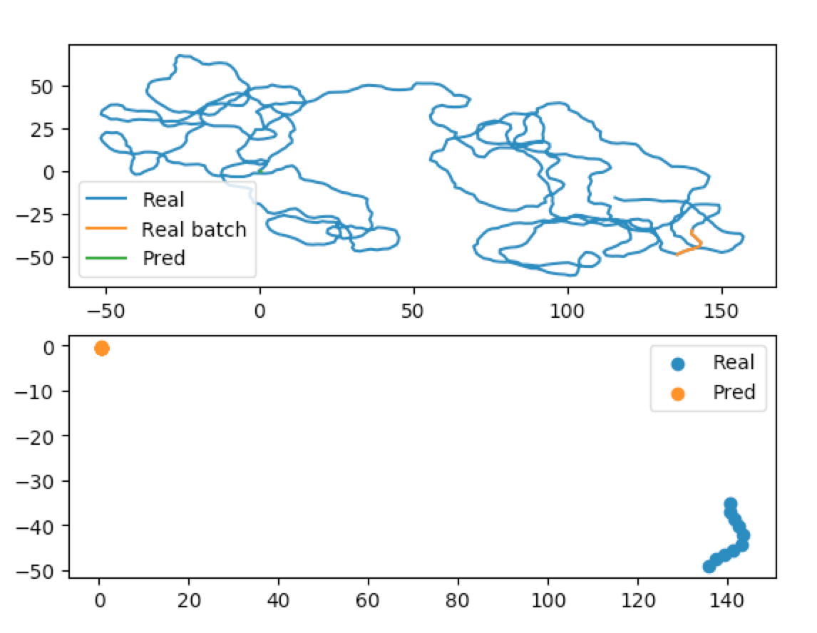
Finally, you can display your training results using the built-in plotting libraries.
from traja.plotting import plot_prediction

batch_index = 0  # The batch you want to plot
plot_prediction(model, validation_loader, batch_index)
Parameter searching
When optimising neural networks, you often want to change the parameters. When training a forecaster, you have to reinitialise and retrain your model. However, when training a classifier or regressor, you can reset these on the fly, since they work directly on the latent space of your model. VAE models provide utility functions to make this easy.
from traja.models import MultiModelVAE
input_size = 2 # Number of input dimensions (normally x, y)
output_size = 2 # Same as input_size when predicting
num_layers = 2 # Number of LSTM layers. Deeper learns more complex patterns but overfits.
hidden_size = 32 # Width of layers. Wider learns bigger patterns but overfits. Try 32, 64, 128, 256, 512
dropout = 0.1 # Ignore some network connections. Improves generalisation.

# Classifier parameters
classifier_hidden_size = 32
num_classifier_layers = 4
num_classes = 42

# Regressor parameters
regressor_hidden_size = 18
num_regressor_layers = 1
num_regressor_parameters = 3

model = MultiModelVAE(input_size=input_size,
                      hidden_size=hidden_size,
                      num_layers=num_layers,
                      output_size=output_size,
                      dropout=dropout,
                      batch_size=batch_size,
                      num_future=num_future,
                      classifier_hidden_size=classifier_hidden_size,
                      num_classifier_layers=num_classifier_layers,
                      num_classes=num_classes,
                      regressor_hidden_size=regressor_hidden_size,
                      num_regressor_layers=num_regressor_layers,
                      num_regressor_parameters=num_regressor_parameters)

new_classifier_hidden_size = 64
new_num_classifier_layers = 2

model.reset_classifier(classifier_hidden_size=new_classifier_hidden_size,
                       num_classifier_layers=new_num_classifier_layers)

new_regressor_hidden_size = 64
new_num_regressor_layers = 2
model.reset_regressor(regressor_hidden_size=new_regressor_hidden_size,
                      num_regressor_layers=new_num_regressor_layers)