Resampling Trajectories
Rediscretize
Rediscretize the trajectory into consistent step lengths with rediscretize() where the R parameter is
the new step length.
Note
Based on the appendix in Bovet and Benhamou, (1988) and Jim McLean’s trajr implementation.
Resample time
resample_time() allows resampling trajectories by a step_time.
- traja.trajectory.resample_time(trj: TrajaDataFrame, step_time: str, new_fps: bool | None = None)[source]
Returns a
TrajaDataFrameresampled to consistent step_time intervals.step_timeshould be expressed as a number-time unit combination, eg “2S” for 2 seconds and “2100L” for 2100 milliseconds.- Parameters:
- Results:
trj (
TrajaDataFrame): Trajectory
>>> from traja import generate, resample_time
>>> df = generate()
>>> resampled = resample_time(df, '50L') # 50 milliseconds
>>> resampled.head()
                                 x         y
time
1970-01-01 00:00:00.000   0.000000  0.000000
1970-01-01 00:00:00.050   0.919113  4.022971
1970-01-01 00:00:00.100  -1.298510  5.423373
1970-01-01 00:00:00.150  -6.057524  4.708803
1970-01-01 00:00:00.200 -10.347759  2.108385
For example:
In [1]: import traja

# Generate a random walk
In [2]: df = traja.generate(n=1000) # Time is in 0.02-second intervals

In [3]: df.head()
Out[3]:
          x         y  time
0  0.000000  0.000000  0.00
1  1.225654  1.488762  0.02
2  2.216797  3.352835  0.04
3  2.215322  5.531329  0.06
4  0.490209  6.363956  0.08
In [4]: resampled = traja.resample_time(df, "50L") # 50 milliseconds
In [5]: resampled.head()
Out[5]:
x y
time
1970-01-01 00:00:00.000 0.000000 0.000000
1970-01-01 00:00:00.050 0.999571 4.293384
1970-01-01 00:00:00.100 -1.298510 5.423373
1970-01-01 00:00:00.150 -6.056916 4.874502
1970-01-01 00:00:00.200 -10.347759 2.108385
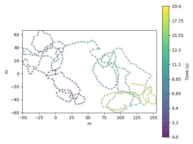
In [6]: fig = resampled.traja.plot()
Ramer–Douglas–Peucker algorithm
Note
Graciously yanked from Fabian Hirschmann’s PyPI package rdp.
rdp() reduces the number of points in a line using the Ramer–Douglas–Peucker algorithm:
from traja.contrib import rdp

# Create dataframe of 1000 x, y coordinates
df = traja.generate(n=1000)

# Extract xy coordinates
xy = df.traja.xy

# Reduce points with epsilon between 0 and 1:
xy_ = rdp(xy, epsilon=0.8)


len(xy_)

Output:
317
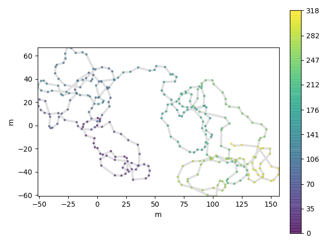
Plotting, we can now see the many fewer points are needed to cover a similar area.:
df = traja.from_xy(xy_)
df.traja.plot()